q2 Code
#contingency table
tab <- matrix(c(85,15,
                60,40,
                35,65),
              nrow = 3, byrow = TRUE)
rownames(tab) <- c("Low","Moderate","High")
colnames(tab) <- c("Achieved","NotAchieved")
tab

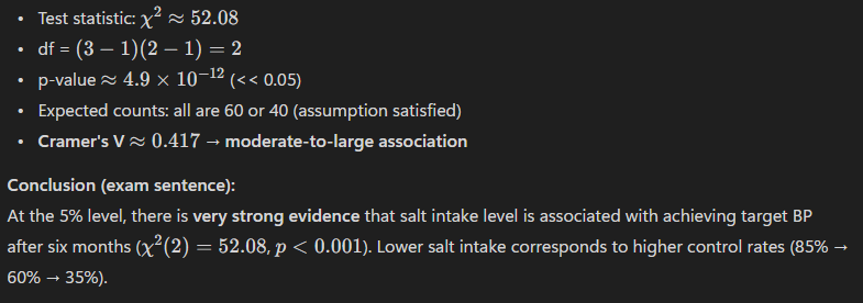
#Chi-square test of independence 
chi_out <- chisq.test(tab, correct = FALSE)
chi_out

#expected counts 
chi_out$expected

#Q2 (b) ANS
low_high <- tab[c("Low","High"), ]
fisher.test(low_high)   # reports OR and 95% CI

2 (a)

[put value according to your output in the r terminal]

2(b)

q3 Code

tab <- matrix(c(145, 25,
                80,  50),
              nrow = 2, byrow = TRUE,
              dimnames = list(
                Before = c("Willing","NotWilling"),
                After  = c("Willing","NotWilling")
              ))
tab

# McNemar’s test (with continuity correction)
mc_out <- mcnemar.test(tab, correct = TRUE)
mc_out

q4 Code

tab <- matrix(c(18, 6,
                8, 22),
              nrow = 2, byrow = TRUE,
              dimnames = list(Sequence = c("AB","BA"),
                              Direction = c("A_gt_B","B_gt_A")))
tab

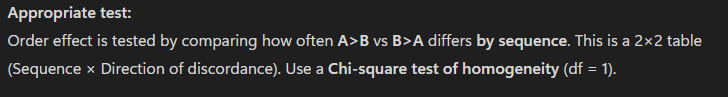
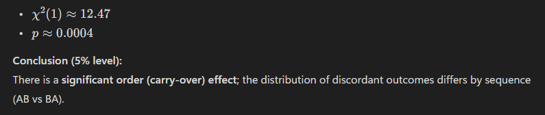
# Chi-square test for order (carry-over) effect
chi_out <- chisq.test(tab, correct = FALSE)
chi_out

# q1_ans

# Load necessary libraries
# install.packages(c("tseries", "forecast"))
library(tseries)
library(forecast)

# data
raw_data <- scan("C:/Users/hp/Desktop/4th year Final Practical exam 2024/88125/411/Q1-411.txt")

# Time Series object
unemployment_ts <- ts(raw_data, start = c(2000, 1), frequency = 12)
View(unemployment_ts)

# (i) Plot Time Series
plot(unemployment_ts, main="Monthly Unemployment Status", ylab="Unemployment", xlab="Time", col="blue", lwd=2)
# Comment: The series shows a visible trend and non-constant mean, indicating non-stationarity.

# (ii) ACF Plot
acf(unemployment_ts, main="ACF of Raw Data")
# Comment: ACF decays very slowly, confirming non-stationarity.

# (iii) ADF Test
adf_test <- adf.test(unemployment_ts)
print(adf_test)
# If p-value > 0.05, it is non-stationary.

# (iv) Transformation (Differencing)
diff_ts <- diff(unemployment_ts)
plot(diff_ts, main="First-Differenced Time Series", ylab="Differenced Value", col="red")
adf_diff <- adf.test(diff_ts)
print(adf_diff) # Verify stationarity

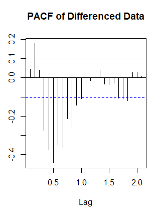
# (v) ACF and PACF for Model Selection
par(mfrow=c(1,2))
acf(diff_ts, main="ACF of Differenced Data")
pacf(diff_ts, main="PACF of Differenced Data")
par(mfrow=c(1,1))

# (vi) & (vii) Fit Model and Diagnostic
# Using auto.arima for best fit based on AIC
best_model <- auto.arima(unemployment_ts, seasonal = FALSE)
summary(best_model)

# Model Diagnostics
checkresiduals(best_model)

# (viii) Forecast next 5 time points
forecast_values <- forecast(best_model, h = 5)
print(forecast_values)
plot(forecast_values, main="5-Month Forecast of Unemployment")

# q1_ans

# install.packages(c("tseries", "forecast"))
library(tseries)
library(forecast)

# data
raw_data <- scan("C:/Users/hp/Desktop/4th year Final Practical exam 2024/88125/411/Q1-411.txt")

# Time Series object
unemployment_ts <- ts(raw_data, start = c(2000, 1), frequency = 12)
View(unemployment_ts)

# (i) Plot Time Series
plot(unemployment_ts, main="Monthly Unemployment Status", ylab="Unemployment", xlab="Time", col="blue", lwd=2)

# (ii) ACF Plot
acf(unemployment_ts, main="ACF of Raw Data")

# (iii) ADF Test
adf_test <- adf.test(unemployment_ts)
print(adf_test)
# If p-value > 0.05, it is non-stationary.

# (iv) Transformation (Differencing)
diff_ts <- diff(unemployment_ts)
plot(diff_ts, main="First-Differenced Time Series", ylab="Differenced Value", col="red")
adf_diff <- adf.test(diff_ts)
print(adf_diff) # Verify stationarity

# (v) ACF and PACF for Model Selection
par(mfrow=c(1,2))
acf(diff_ts, main="ACF of Differenced Data")
pacf(diff_ts, main="PACF of Differenced Data")
par(mfrow=c(1,1))

# (vi) & (vii) Fit Model and Diagnostic
# Using auto.arima for best fit based on AIC
best_model <- auto.arima(unemployment_ts, seasonal = FALSE)
summary(best_model)

# Model Diagnostics
checkresiduals(best_model)

# (viii) Forecast next 5 time points
forecast_values <- forecast(best_model, h = 5)
print(forecast_values)
plot(forecast_values, main="5-Month Forecast of Unemployment")